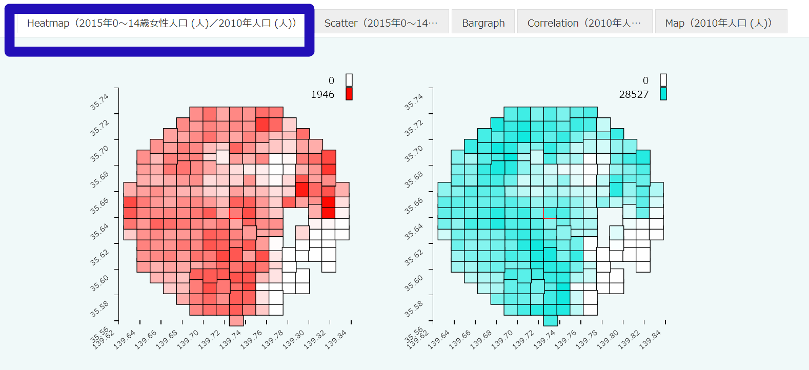
You can select up to two types of data from the list, and make the data matrix of individual values expressed as a color difference.You can compare and display two types of world mesh statistics in the visualization graph. Select "heatmap" from the tab lists if you want to use.
In the following figure, as an example, 2015 female population aged 0-14 and 2010 population are displayed You can compare visually two types of world mesh statistics in the same selected area.
bargraph
Explanation
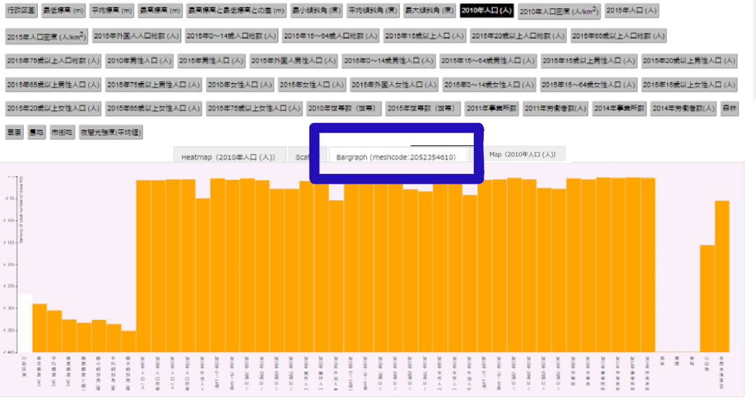
Select one piece of mesh data from the list, and it will draw the bar graph corresponding to all of the data number or quantity of available world mesh statistics. By using the bargraph function, you can understand feature trends and the value of it in the selected area. If you want to use this function, please select bargraph from the tab after identifying features by using heatmap, scatter, or map.
In the following figure, as an example, 2015 female population aged 0-14 and 2010 population are displayed. You can compare visually two types of world mesh statistics in the same selected area.
scatter
Explanation
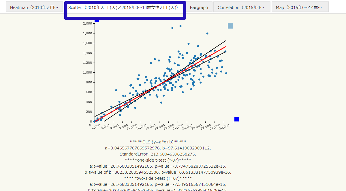
Use this function by selecting two types of mesh statistics from the data list. Data can be plotted in dots and displayed in a scatter, with the vertical and horizontal axes corresponding to up to two different quantities, sizes, etc. Logarithmic conversion of axis values is applied by clicking on a light-blue square on each axis. Also, if you click on a scatter plot point, the world mesh square can be extracted. The extracted mesh is displayed as blue pin on the map. It also appears as all the feature values in the bargraph at the selected world mesh square. The three lines illustrate the results of linear regression analysis. Two straight black lines are OLS regression analysis which explains the y-axis by the x-axis. Parameter estimates of regression analysis are shown below the scatter plots. Statistical significance level of regression coefficients by t-test are displayed. The red line is of RMA regression analysis.The regression coefficients are also displayed at the bottom of the scatter plots. If you want to use it, select scatter from the tab. This function also can be used to detect outliers that tend to be out of place from other scatter plots for finding something interesting.
In the following figure, for example, the 2015 female population (population census) aged 0-14 and the 2010 cencus population have been chosen. Trends per world grid square for two types of selected data can be confirmed visually.
correlation
Explanation
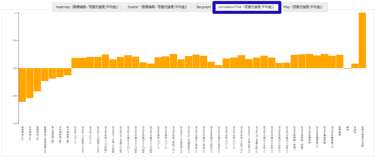
Use this function by selecting one world mesh statistic or datum from the data list. The correlation coefficient of values between selected world mesh statistics or data and others are computed and displayed as bar graphs. The correlation coefficient takes a value between -1 and 1. It represents the closer to 1 a positive values of the correlation coefficient, the more similar the two values tend to be. It represents the closer to -1 a negative values of the correlation coefficient, the more opposite two values tend to be. If the correlation coefficient takes 0, then two values are uncorrelated and have no relationship.
In the following figure, as an example, it represents correlation coefficients between the 2012 night-time light intensity and others. Because there is a negative correlation in the bar graph, a place where night-time light intensity is strong tends to be at lower elevation levels.
map
Explanation
Use this function by selecting one world mesh statistic or datum from the data list. You can display a visualization graph that represents a data matrix of individual values as a color on the map. In the following figure, as an example, you can select the 2010 population (cencus population) to display their values of world mesh statistics on the map. A detailed value are displayed in a pop-up window by selecting a mesh square.